The Eddington experiment and the technical difficulties of the deflection measurement
In 1919, British astronomer Arthur Eddington organized an expedition to observe the total solar eclipse of 29 May 1919 from Sobral in Brazil and Principe Island in Africa. The main objective was to test Albert Einstein theory of general relativity, published just four years before, in 1915. This theory predicted that the star positions in the sky are modified if a big mass lies in the same field of view, like stars during a total solar eclipse. Newton’s gravity theory also predicted a deflection, however the value it yields is half the one resulting from the application of Einstein’s theory. Measuring the deflection would have determined which theory is correct, and would have offered a second experimental proof to the theory (the other already known proof is the precession of the Mercury’s perihelion).
In principle, the gravitational deflection of stars is quite simple. The value of the deflection can be computed with the following simple formula:
d=k/SR
where d is the star deflection in the radial direction (in arcsec), k is a constant that depends on the theory (k=1.752"/pix for Einstein, k=0.875"/pix for Newton), and SR is the distance of the star from the Sun center (in solar radii unit, in short SR).

In practical terms, making such a measurement poses a number of technical challenges. The value of deflection is quite small, only 1.7" at the Sun’s edge. Unfortunately, the sky near the Sun during a total solar eclipse is not as dark as during the night! The Sun’s atmosphere, the corona, is extremely bright especially near the disc’s edge. As a consequence, stars are observable starting from about 1.5 SR, and much better from 3.0 SR. But at these distances, the deflection value reduces to even extremely smaller angles, 1.2" and 0.6" respectively. Please consider that the resolving power of a 140 mm diameter telescope is 0.98" in white light computed using the formula for "Rayleigh’s criterion": R=0.25*lambda/D=0.25*550/140=0.98" where R is resolution in arcseconds, lambda is the light wavelength in nanometers and D is the scope diameter in millimeters. This shows that the resolution of a “typical” telescope is comparable to the value of deflection to be measured.

Fortunately, the position of a star can be measured with better uncertainty than the telescope’s resolving power by interpolating the star brightness profile. In an ideal case, the star position can be determined down to ~0.2 times the angular resolution of the telescope. The ideal case is a star with a very high SNR (signal to noise ratio), i.e. a bright star over a dark background. Good SNR values are around 100 or higher. However, stars near the Sun during an eclipse are by far not an ideal case! Most stars in my eclipse image have a SNR less than 10, and most of them less than 3! In particular, the two stars at 1.5 SR have SNR ~1, i.e. they are even extremely difficult to spot. I was able to locate them in my image only after blinking a noise-filtered image of the eclipse with a star map.

Another big limit is air turbulence, or "seeing". The size of stars depends not only on the resolution of the telescope, but mostly on the seeing. Standard seeing values range between 0.5" to 4", with values in the lower part of the range being found only at very limited locations atop mountain peaks (i.e. Mauna Kea in Hawaii or Paranal in Chile). Moreover, during the day, the seeing values are even worse, ranging from 3" to 10", which is much higher than the deflection values to be measured!
For example, the average FWHM for stars in images taken with my TEC140 is around 2.8" at night and 5" during the eclipse (in the daytime).

All these challenges were encountered during Eddington’s experiment as, and the values obtained from the 1919 expeditions were strongly criticized in 1980. However, most of the astronomical community still agrees that Eddington’s results are not flawed. Moreover, the measurements have been repeated many times and the Einstein’s theory has always provided the best fit for the measured displacements.

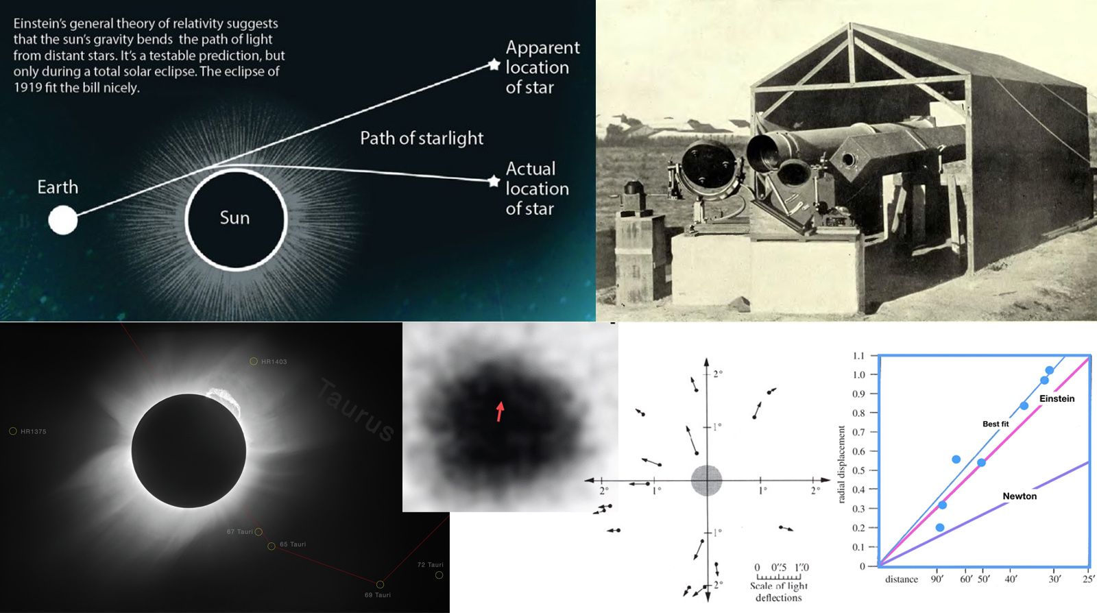
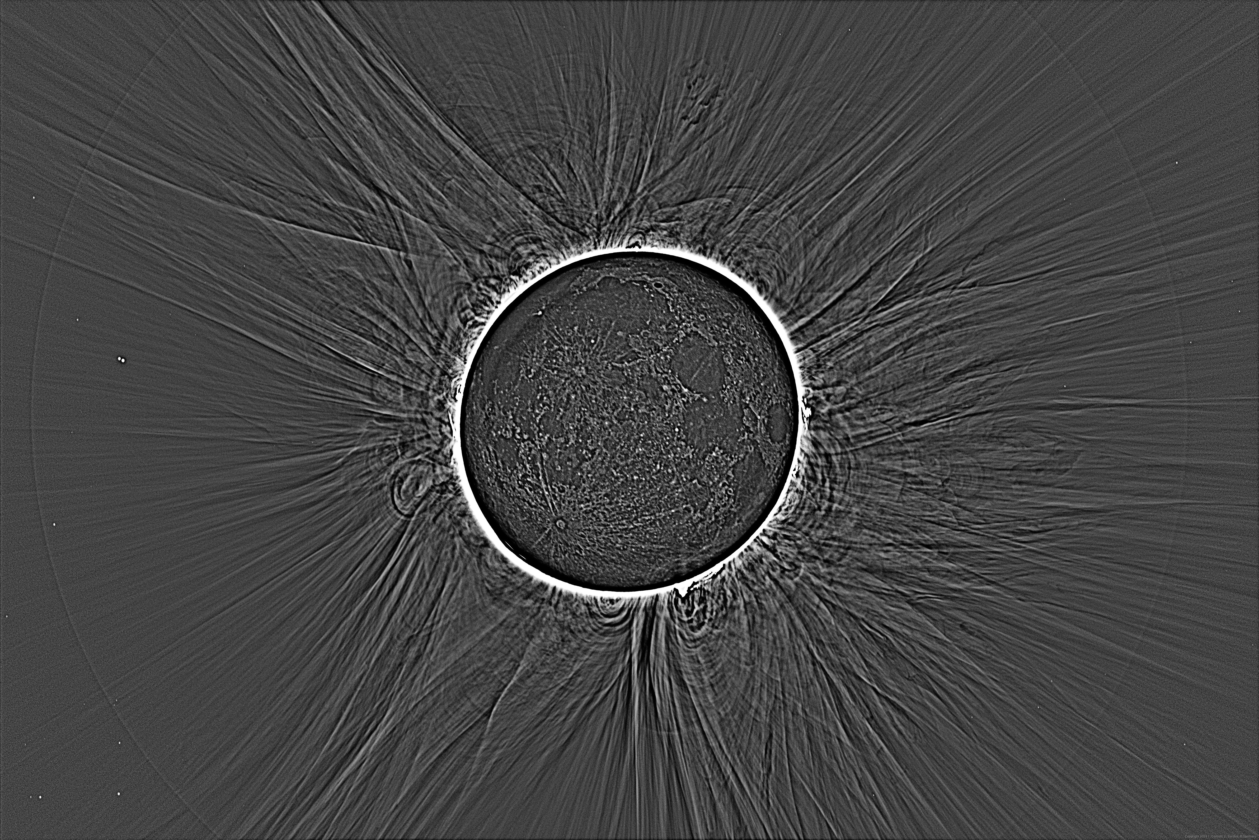
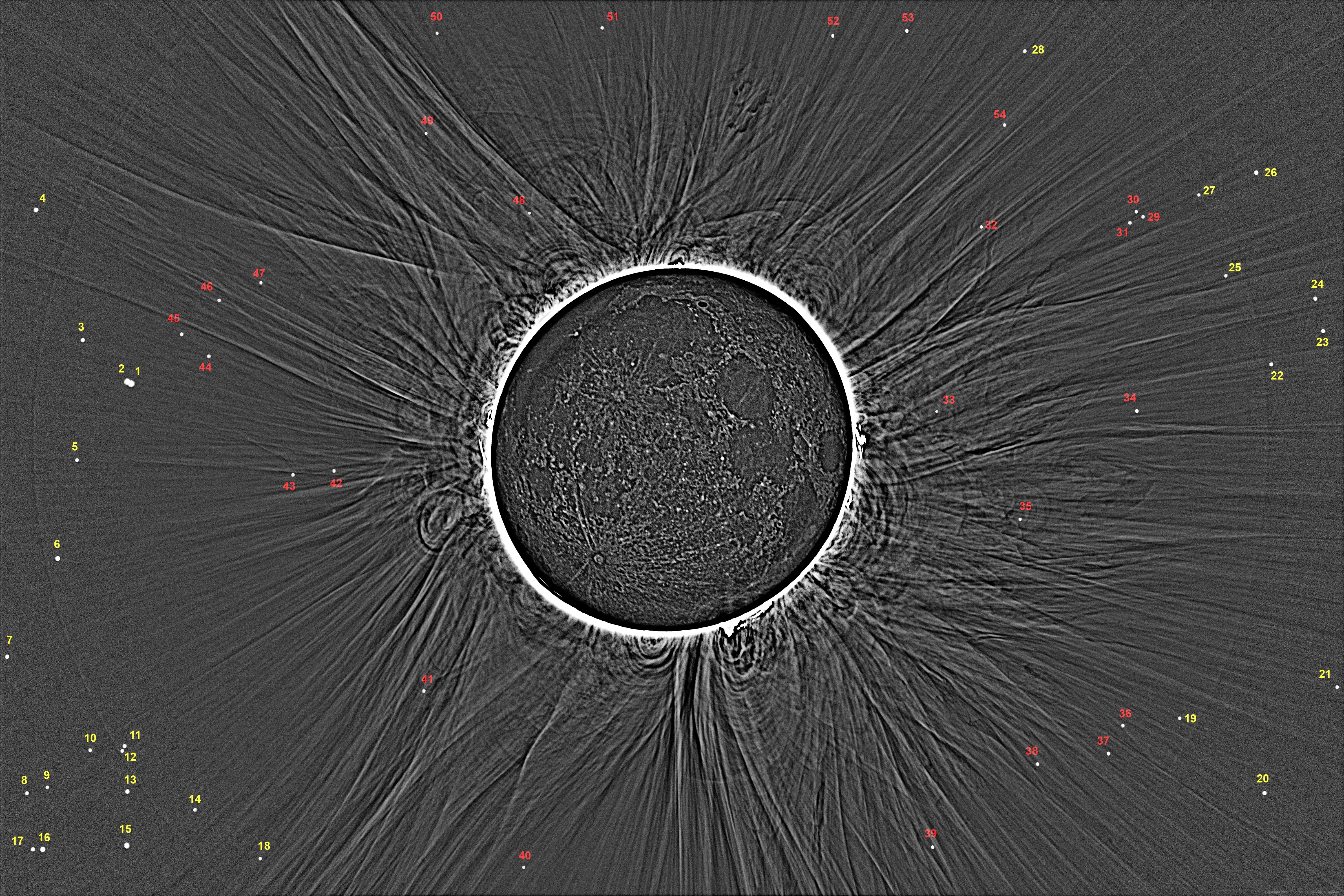
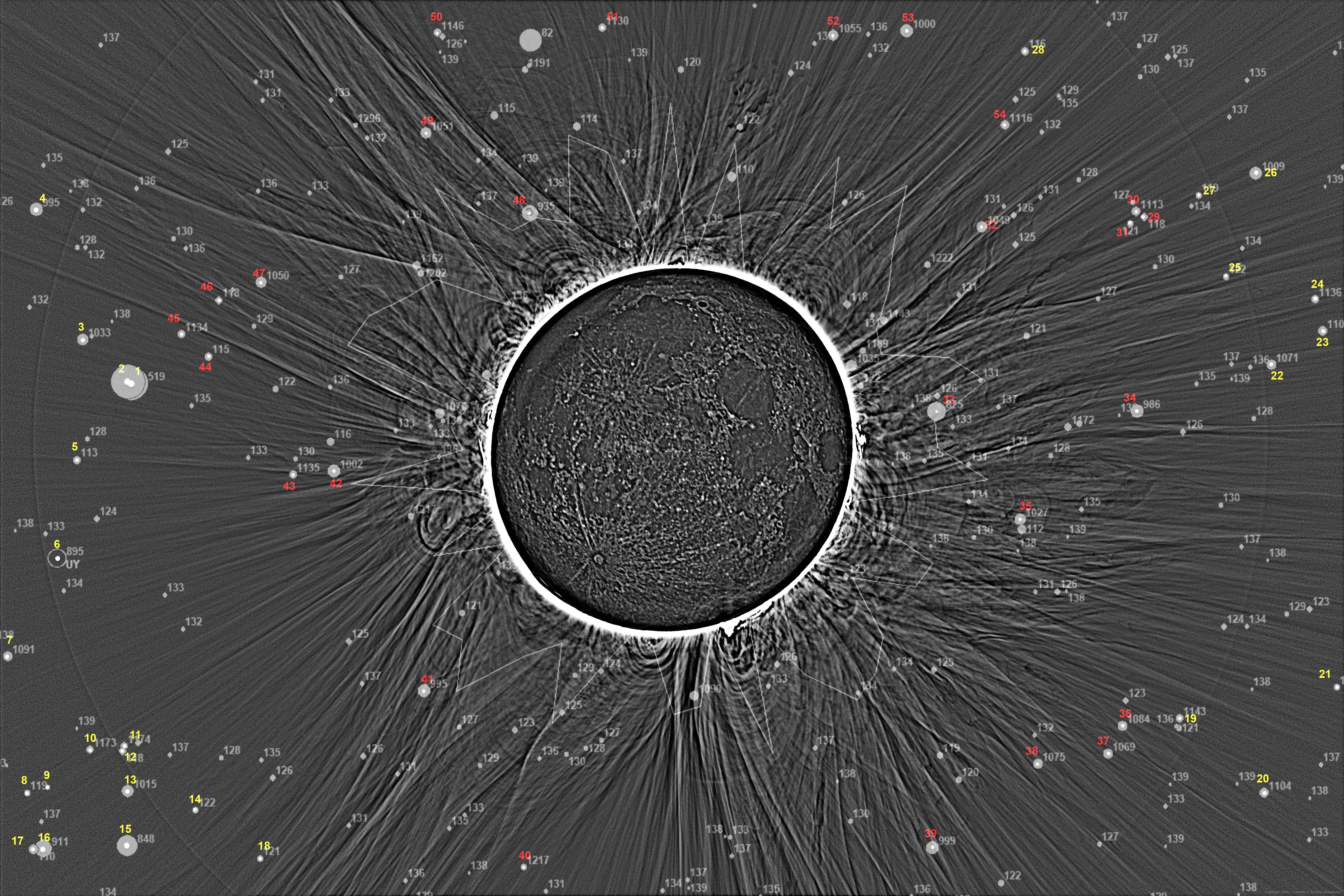
The Eddington experiment of 1919: 1. (top left): graphical explanation of the gravitational deflection of stars during a total solar eclipse 2. (top right): the setup of Sobral, Brazil was a very complicated set of telescopes coupled with heliostat mirrors 3. (bottom left): one of the images taken in 1919 shows may stars thanks to the very lucky fact that a couple of very bright stars are located very close to the Sun’s Edge, i.e. 67 Tau mag 5.2 at 2.0 SR and 65 Tau mag 4.2 at 2.5 SR. 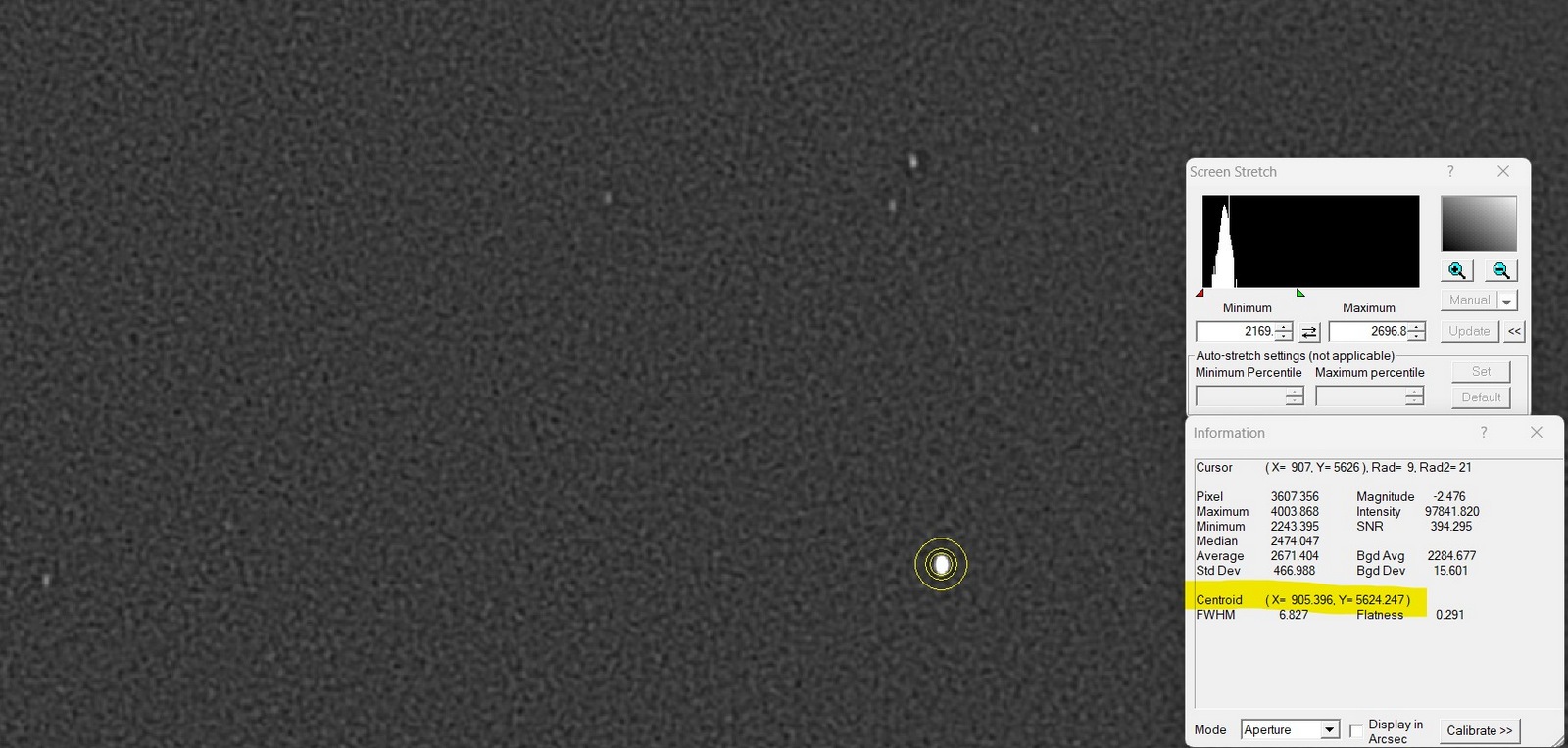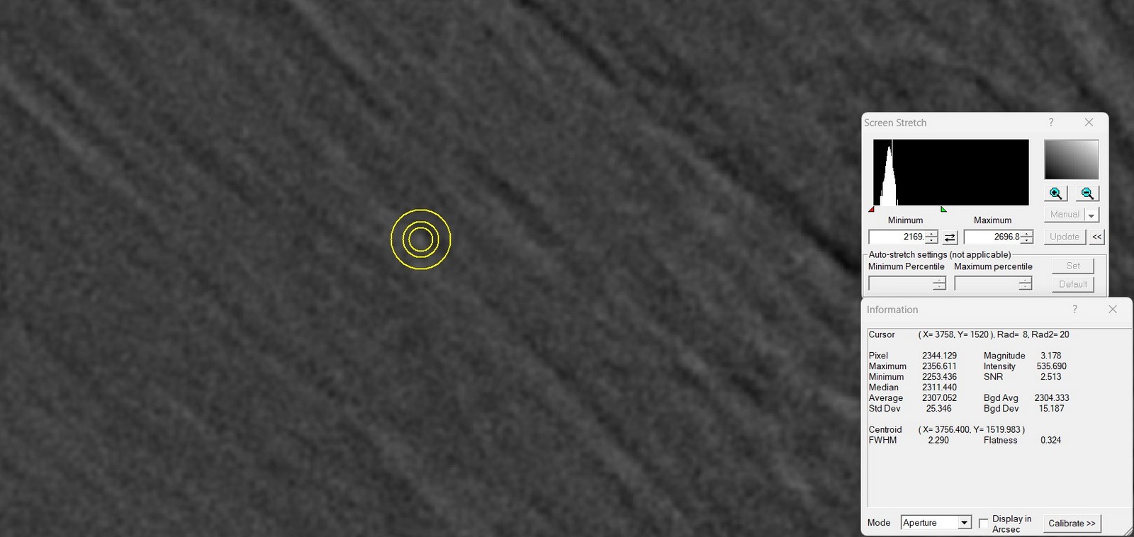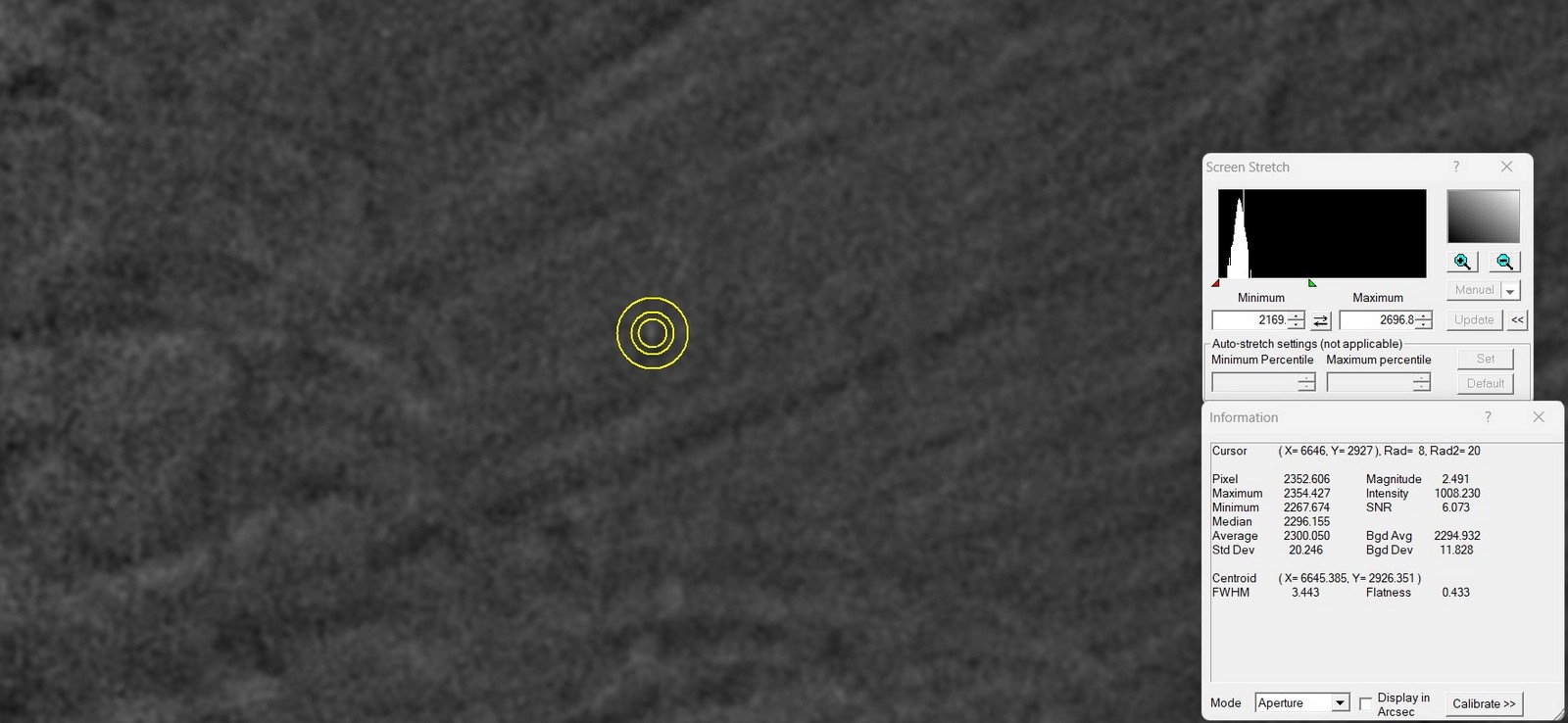4. (bottom center/left): an extreme close-up of a star together with an arrow showing the theoretical deflection value. This clearly shows how difficult the measurement was, because the deflection value is far smaller than the star diameter itself! Star 4, arrow represents a 0.75" deflection. 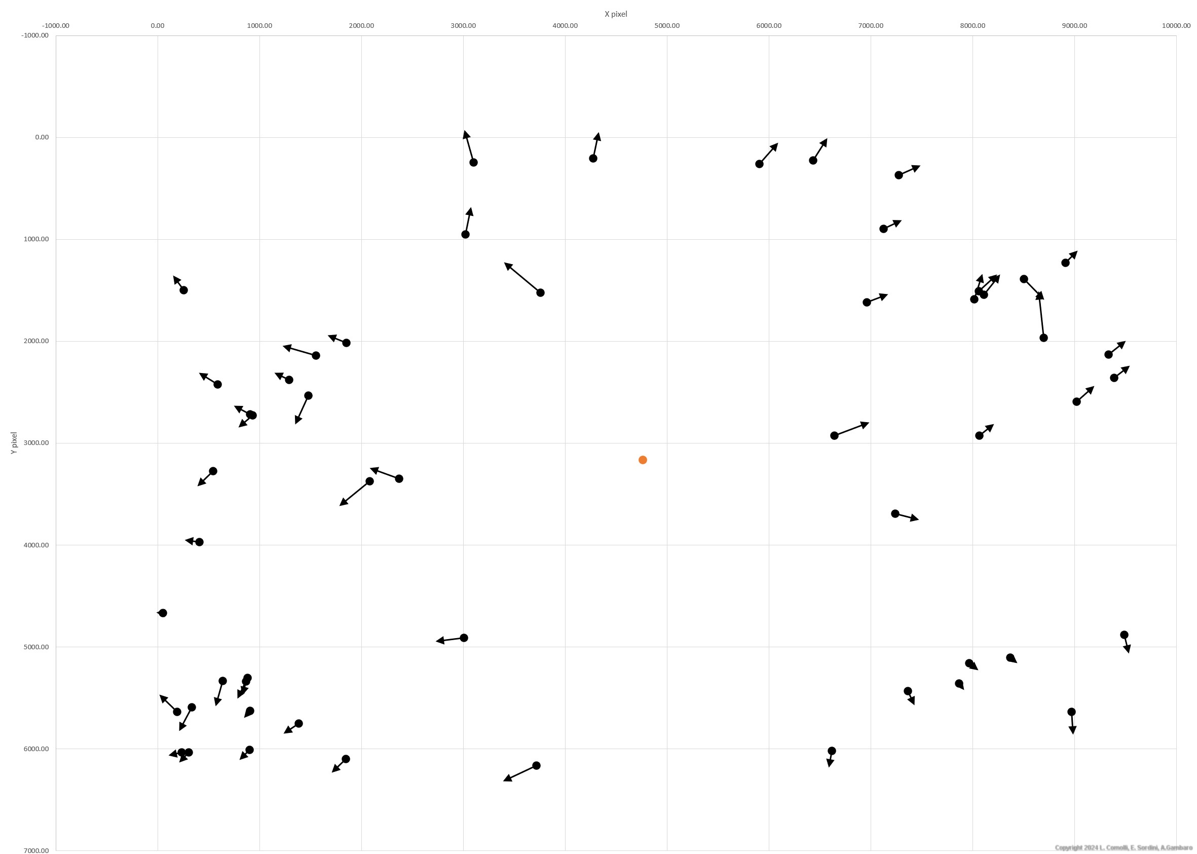5. (bottom-center/right): arrow plot of measured deflections in the 1922 eclipse from Australia by astronomers W. W. Campbell and R. J. Trumpler 6. (bottom-right): graph of the measured deflections in 1919 compared to theoretical predictions Image credits: 1. GSFC/NASA 2. This photo by Charles Davidson is provided courtesy of Graham Dolan. 3. This image is from a PDS (Photometric Data Systems) machine scan of an eclipse plate made by John Pilkington at the Royal Greenwich Observatory in 1999, at the request of and kindly provided by Dr Robin Catchpole 4. CC BY 4.0 ESO/Landessternwarte Heidelberg-Königstuhl/F. W. Dyson, A. S. Eddington, & C. Davidson - https://www.eso.org/public/images/potw1926a/ 5. figure from Misner et al, Gravitation, Freeman and Co., 1973, 1104 6. Enhanced version of diagram 2 from Dyson et al. 1920, https://eclipse1919.org/index.php/the-expeditions/11-announcing-the-results

Results from my data
A graphical result of my work is the below arrow plot of all the visible stars. The arrows are superimposed on the HDR of corona. If the reader is interested only in aesthetically pleasing pictures, then I recommend taking a look at our main eclipse page. Most of the stars show arrows pointing away from the Sun’s center (blue dot), with a radial amplitude nearly proportional to the distance from the Sun. The arrow length is increased by 250 times the measured value because otherwise they would not be noticeable. Some stars show also circumferential deflections, which are clearly measurement errors but give an idea of the measurement uncertainty. Stars #33 and #48 at 1.5 SR distance shine at mag. 8.8 and 9.4 respectively; they are barely visible, but can be spotted more easily by blinking the image with a star map.

Another interesting result is the plot of radial deflections as a function of the distance from the Sun (see graph below). In this graph, stars clearly follow a trend indicated by the orange dotted line, which is produced the interpolation of all the stars with good SNR.
My data yield a value for the constant k of 1.93 " +/- 0.18" (confidence interval 68%), which is in good accordance with that from Einstein’s theory of 1.752 ".

Click on the image for high res version. MOUSE OVER for deflection arrows. Look also to the Arrows without HDR hires.

Arrows plot of the measured deflections. Most of the stars show arrows pointing away from the Sun’s center (blue dot), with a radial amplitude nearly proportional to the distance from the Sun. The arrow length is increased 250 times the measured value.

Graph of radial deflections of stars in arcseconds versus the distance from the Sun center in solar radii units. Brighter stars are orange circles while fainter ones are light blue. Theoretical behaviors are depicted with a red curve for Einstein’s theory; the blue curve represents Newton’s theory. The orange dotted curve is the result of the interpolation of brighter stars in my image.

Measurement method
Here is a description of the method I used to compute the deflections.

First of all, I excluded the method typically used for astrometric measurements of asteroids, i.e. plate solving using software like Astrometrica. Unfortunately, plate solving does not work on eclipse images because of missing stars in the center of the frame and also because most of the stars are so faint that the automatic algorithms cannot spot them. Additionally, plate solving needs to evaluate the field geometrical distortions and this would compensate the gravitational distortions to be measured.

Consequently, I used a method quite similar to the one used by Eddington in 1919, i.e. comparing star positions in the eclipse image with positions of the same stars in the same star field imaged exactly with the same setup a few months before or after eclipse day. This way, optical distortions of the focal plane are automatically compensated.

However, I was faced with a big problem I've never encountered in my 30-plus years career as an astrophotographer: the focal length of any telescope changes with temperature. But the reason for this is not the most obvious one, i.e. thermal expansion of the optical tube, which can be easily tamed by focusing on the subject a few minutes before imaging. The reason is much more subtle, and in case of a refractor like my TEC140 it comes from the change in the refraction index of the lens glass with temperature.
Here is a practical example: my scope has a focal length (FL in short) of about 1017 mm, a little higher than the “nominal” 980 mm because I was using the TEC field corrector which extends the FL by a few percent. I measured the real FL using the eclipse star field on two dates:

• 12 Jan 2024, air temperature -3.1°C, image scale 0.763138 "/pix, FL=1016.273 mm
• 18 Jul 2024, air temperature +22.8°C, image scale 0.762270 "/pix, FL= 1017.430 mm

The above image scale was computed using Astrometry.org, while the FL was then computed with the following simple formula:
FL=206265*PIX/S
where FL is the focal length in millimeters, PIX is the pixel size of the camera in micrometers per pixel (mine is an ASI6200MM yielding 3.76 um/pix) and S is the image scale in arcseconds per pixel.
So, I found a focal length change of 1.157 mm for a temperature change of 25.9°C, giving a coefficient of 44.7 um/°C.

The temperature during the max of eclipse was 27.5°C (see temperature logging on the main eclipse page) so I figured out the image scale to be 0.762112 "/pix with FL=1017.641 mm.
Subsequently, I computed the scale ratio between the 12 Jan 2024 reference and the eclipse image (1.00135), a very small difference of about 0.1%, which however is absolutely fundamental for obtaining a reliable estimate of the gravitational deflections.

I found that this scale ratio is the most critical parameter, so for sure the next time I do this experiment I will need to get a more precise image scale measurement. I think that the simplest and most reliable way is to measure the image scale by taking a shot of a star field immediately after totality (when the sky is not too bright), or even during totality by slewing the telescope to another position, e.g. at 10-30° from the Sun. At this angular distance, the gravitational deflection effect is negligible. And by taking this image a few minutes after the eclipse image, the temperature of the telescope will be exactly the same, and so will be the FL and the image scale.

Focal length change with temperature of my telescope, TEC140 with field flattener and ASI6200MM camera. Even if it seems a very small change, it is of fundamental importance when measuring the extremely small gravitational deflection of stars during an eclipse.

The method I used is to measure centroids for a selection of 54 stars found in the image below. This image is obtained by removing the large-scale light gradient from the solar corona. The image was produced simply by subtracting from the HDR image a copy where I removed the stars by using a 10 pixel radius gaussian blur. In this image, small-scale details of the corona are also visible even if they are not needed for the task. This also gives an idea of how deep the obtained HDR image of the corona is.

Star centroids were measured using Maxim DL software. Maxim’s centroid measurement algorithm is not very sophisticated but I found it to be very reliable for extremely faint stars. The algorithm uses 2D interpolation of a gaussian curve of the light profile in the X and Y directions: these light profiles are obtained by summing pixel values in the Y and X directions respectively. Modern interpolation algorithms use 3D interpolation of a bivariate gaussian distribution, but I found that they fail on very faint stars with SNR<3.
Moreover, for improving the reliability and reducing the uncertainty of star centroid values, I slightly defocused the star field with a gaussian filter of 1.5 pixel radius. This greatly enhanced the visibility of extremely faint stars.

A mystery and call for ideas: in this image a large circle with a diameter of about 90% of the width of the image is also visible. I have no idea whatsoever of the reason for this. Please note that the images were dark and flat calibrated and in the master flat field there is no evidence of such a structure. The circle is literally perfectly circular, so it is not something related to the brightness profile of the corona, which is not perfectly circular itself. It may be a kind of reflection from some optical surface, but I've never found anything like that in my long-time experience as an owner of this telescope. Another possibility could be something on the Sony IMX455 CMOS sensor. I also noticed that it is not perfectly centered with respect to both the Sun’s center and the sensor’s center. If you have the solution to this mystery, please drop me a line!

Click on the image for high res version. MOUSE OVER for star numbers. Look also to the Star Numbers hires and Magnitudes from Guide8 hires.

The HDR image from TEC140+ASI6200MM setup was processed to remove the large-scale structures of the corona, so to "flat field" the background sky. The image processing technique is very simple: from the HDR image I subtracted a gaussian blurred copy with a 10 pixel radius. This way, stars are more easily visible and measurable. I counted 54 visible stars in the field: numbers were assigned in an arbitrary order. Some of them are very hard to spot, especially the stars #33 and #48 are at 1.5 SR and are mag. 8.8 and 9.4 respectively.

Measurement of the centroid of star #13 from a defocused version of the above image (in the lower left corner) using Maxim DL. Centroid values are a little different from the ones used in the table because they were remeasured for the screenshot purpose a month later, so probably using slightly different settings. SNR is much higher compared to the table below because this measurement is on the gaussian blurred image, while the SNR reported in the table comes from the original image.

Star #48 at 1.5 SR was extremely difficult to measure even on this defocused version. Moreover, the star is superimposed to a small corona wisp. Centroid values are a little different from the ones used in the table because they were remeasured for the screenshot purpose a month later, so probably using slightly different settings. SNR is much higher compared to the table below because this measurement is on the gaussian blurred image, while the SNR reported in the table comes from the original image.

Star #33 at 1.5 SR was also extremely difficult to measure. Centroid values are a little different from the ones used in the table because they were remeasured for the screenshot purpose a month later, so probably using slightly different settings. SNR is much higher compared to the table below because this measurement is on the gaussian blurred image, while the SNR reported in the table comes from the original image.

The below table is the Excel spreadsheet used to compute star deviations and alignment coefficients. In the first columns (B to E) I entered the pixel coordinates of the star centroids as measured in Maxim DL on the reference image ("out of eclipse", taken on 12 Jan 2024) and on the eclipse HDR image ("in eclipse"). Also, the SNR is reported as measured in the not blurred "in eclipse" image (column F); this value is used to filter the interpolation only on stars with decent SNR (e.g. SNR>5).

The pixel coordinates of "out of eclipse" stars have been aligned to the "in eclipse" image by a scale-roto-translation by using as a scale coefficient the one determined using the FL vs temperature coefficient (cell H19), and the 3 roto-translation coefficients (cells F19, G19, I19) obtained using the Solver function in Excel with the objective to have minimum MSE (mean squared error, cell AD21)) from the differences of "in" and "out" of eclipse pixel coordinates (columns U and V).

A check of the image alignment was performed without considering the above fixed image scale, and the results are in the gray cells (columns from G to R). However, this alignment was not used in the computation of the deflections.

Star deflections are computed (column AA) and interpolated with a curve. The only coefficient of this curve is the deflection at 1 SR, and this was computed with Solver in Excel by obtaining the minimum MSE of the differences between the measured deflections and the interpolation deflections (cell AF21). This gave a result of 1.93 " (cell AE21). The uncertainty of this value is also computed by the square root of the MSE, i.e. ME=0.18 " (cell AF19).

Finally, I computed the pixel coordinates of the start and end points of the arrows for the "arrow plot" (columns AH to AK). These values were then plotted with an Excel macro I developed by modifying a sample macro from the Internet.

Table of all the measurements and calculations for the deflection value. See the above description for details.

Conclusions
I think that it is amazing to see that amateur astronomers can now reproduce Eddington’s experiment with a simple setup like the one described in this article. Now in 2024, amateurs with a 10000 € setup and a 2000 € trip can get better results than what was obtained back in 1919 by Eddington, the most famous astronomer in the world at the time, who had professional equipment at his disposal and dozens of experienced astronomers working for years on the preparation of this experiment. Progress made in 105 years of technological evolution can make a huge difference!

I really hope to repeat the measurement during the next eclipse of 2027. Meanwhile, I hope you enjoyed my article. Please email me at comolli@libero.it for any comments or criticisms, both of which would be greatly appreciated!


Acknowledgements
I'd like to thank my friends Emmanuele and Alessandro for sharing the expedition for the eclipse, for the comments and in particular Emmanuele for revision of the first draft of English text.